
AI demand forecasting: a step-by-step guide for fashion retail
In fashion, product lifecycles are short, most products have no history, and size and colour split demand. How AI demand forecasting is built in fashion retail in seven steps, and how it attaches to decisions.
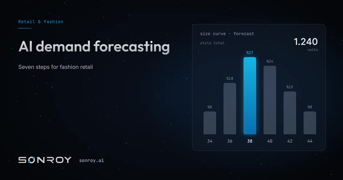
AI demand forecasting means predicting demand with machine-learning models that read sales history together with signals such as price, promotions, returns, stock, weather and search trends, and attaching that forecast to order, catalog and budget decisions. Fashion retail is exactly where classical methods struggle.
Why is demand forecasting hard in fashion retail?
For four reasons. Lifecycles are short; a style sells for one season and never returns, so most products have no history of their own. Demand splits by size and colour; one style spreads across fifteen or twenty stock units, and each one's volume shrinks. Finally, observed sales do not show true demand: when a size sells out, that week's sales look low, but demand did not fall. The basic methods of demand forecasting are not enough on their own under these conditions.
Step 1: Bring the data into one memory
Sales sit in the ERP, e-commerce orders on the platform, marketplace sales in a separate panel, store sales at the till, returns in yet another system. The forecast must see all of them under the same product identity. SNR Core leaves existing systems in place and joins their data in one company memory; the forecast reads from that memory.
Step 2: Forecast at the right level
Forecasting directly at size and colour level is noisy because the volumes are small. The sturdier route is to forecast demand at product group, channel and week level, then distribute it with a size curve. S0 Forecast's Size Curve module forecasts the size distribution separately, so a style's total demand and how many units of each size it needs are answered as two separate questions.
Step 3: Learn products without history from similar ones
A new style has no history, but it has look-alikes: same category, same price band, similar fabric, similar fit. The model forecasts the new product from how those look-alikes behaved in their first weeks. That requires clean product attributes; we covered where product data comes from in Pimland and SONROY. In S0 Forecast this is the job of the New Product Forecast module.
Step 4: Add external signals and the calendar
Weather, market movement and search trends show what sales history cannot. The promotion and season calendar is part of the forecast too; a markdown week cannot be forecast with the same model as an ordinary week. In S0 Forecast, Trend Signals brings external signals into the forecast and Season Calendar brings the season and promotion calendar.
Step 5: Correct for out-of-stock weeks and returns
In weeks when a size is sold out, observed sales sit below true demand; the model must not mistake those weeks for falling demand. Returns are part of demand as well: a size with high returns means less net demand than its sales figure suggests. We covered the level at which to read returns in how return data becomes a production decision.
Step 6: Attach the forecast to a decision
A forecast that stays on a screen is worth nothing. The forecast flows to S0 Supply as an order proposal, to S0 Ecom as a catalog plan and to S0 Finance as a budget. The planner sees the recommendation with its reasoning and approves or rejects it. An approved order goes to the supplier.
Step 7: Measure deviation and let the model correct itself
Every period, actual sales are compared with the forecast. The Forecast Accuracy module tracks deviation by product, category and channel, and the model is updated with that gap. Rejected recommendations are recorded too: over time it becomes visible where the planner was right and where the model was.
How does AI differ from the classical approach?
| Classical demand forecasting | AI demand forecasting | |
|---|---|---|
| Input | Mostly sales history | Sales, returns, stock, price, promotions, weather, search trends |
| New products | Expert estimate | Forecast from similar products' behaviour |
| Sizes | Split with fixed ratios | A separately forecast size curve |
| Updating | Periodic, manual | Every period, from deviation |
| Output | A report | A reasoned order and plan recommendation |
Where do you start?
Pick one product group and one decision; for most teams the best start is the weekly reorder, because its outcome is measured within a few weeks. To see this flow on your own sales and return data, book a demo.
Short answers
The history of the product group and of similar products matters more than the product's own past. Having sales, return and stock data joined under the same product identity is more decisive than the amount of data.
A new style is forecast from how similar products in the same category, price band and attributes behaved in their first weeks. That requires clean, consistent product attributes.
The planner. The system brings the recommendation with its reasoning; the planner approves or rejects it. An approved order goes to the supplier, and the outcome is measured and written back to the model.
Summary
- In fashion, lifecycles are short, most products have no history and demand splits by size and colour.
- Demand is forecast at product group, channel and week level, then distributed with a size curve.
- A forecast that does not correct for out-of-stock weeks and returns misstates demand.
- The forecast attaches to order, catalog and budget decisions; deviation is measured every period.
Related
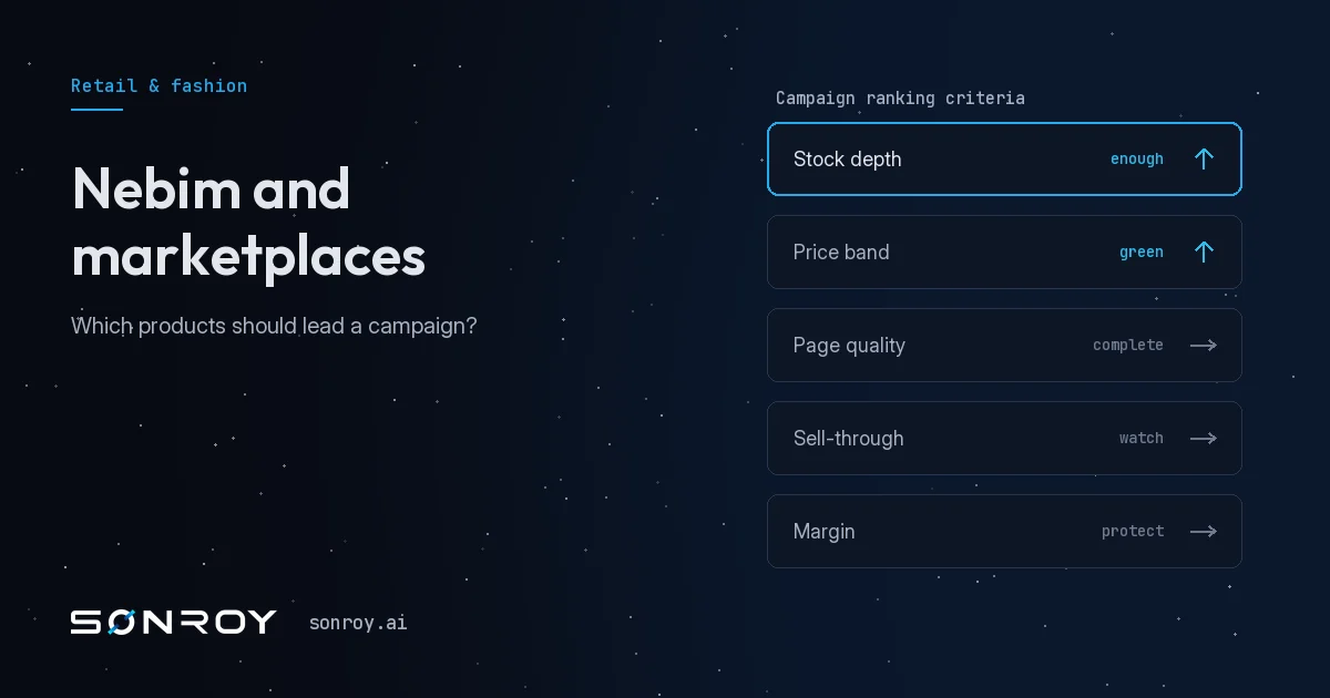
Nebim and marketplaces: which products should lead a campaign?
Which products go on the first page during a campaign is a decision made by reading stock and sales in Nebim together with competitor prices and customer questions on the marketplace. A decision flow and checklist for campaign product selection.
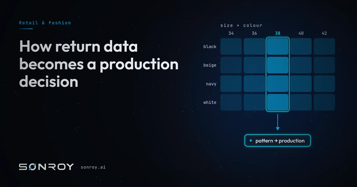
How return data becomes a production decision
The size × colour return matrix is not a report; it is a production instruction. The level at which returns should be read in fashion retail, three different causes, three different owners, and the path from that level to action.
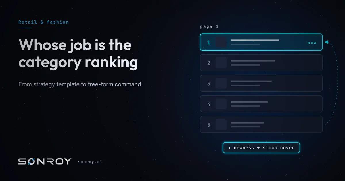
Whose job is the category ranking: from strategy template to free-form command
Deciding which product sits on the first page of an e-commerce category used to take a person days. How strategy templates and free-form commands reduced that work to one command, and where the category specialist's job moved.